
NeuroFlow is a Scala library to design, train and evaluate Artificial Neural Networks.
- Getting started
- Construct a Dense Net
- Training it
- Monitoring
- Evaluation
- Extending
- Using GPU
- Persistence
The library aims at ease of use, keeping things intuitive and simple. Neural Nets bring joy into your project, a journey full of experiments. :o)
There are three modules:
- core: building blocks for neural networks
- application: plugins, helpers, functionality related to application
- playground: examples how to use it
To use NeuroFlow for Scala 2.12.x, add these dependencies to your SBT project:
libraryDependencies ++= Seq(
  "com.zenecture"   %%   "neuroflow-core"          %   "1.8.2",
  "com.zenecture"   %%   "neuroflow-application"   %   "1.8.2"
)

resolvers ++= Seq(
  "neuroflow-libs" at "https://github.com/zenecture/neuroflow-libs/raw/master/"
)
If you are new to the math behind Neural Nets, you can read about the core principles here:
Seeing code examples is a good way to get started. You may have a look at the playground for basic inspiration.
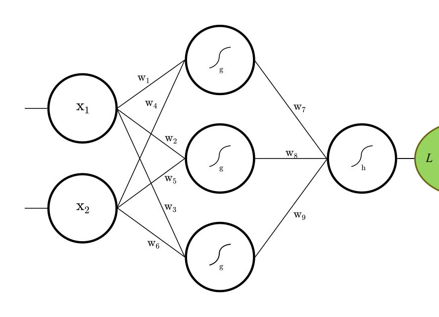
Let's construct the fully connected feed-forward net (FFN) depicted above.
import neuroflow.application.plugin.Notation._
import neuroflow.core.Activators.Double._
import neuroflow.core._
import neuroflow.dsl._
import neuroflow.nets.cpu.DenseNetwork._

implicit val weights = WeightBreeder[Double].normal(μ = 0.0, σ = 1.0)

val (g, h) = (Sigmoid, Sigmoid)

val L = Vector(2) :: Dense(3, g) :: Dense(1, h) :: SquaredError()

val net = Network(
  layout = L,
  settings = Settings[Double](
    updateRule = Vanilla(),
    batchSize = Some(4),
    iterations = 100000,
    learningRate = {
      case (iter, α) if iter < 128 => 1.0
      case (_, _)  => 0.5
    },
    precision = 1E-4
  )
)
This gives a fully connected DenseNetwork under the SquaredError loss function, running on CPU. The weights are drawn from
normal distribution by WeightBreeder. We have predefined activators and place a softly firing Sigmoid on the cells. Layout L is
implemented as a heterogenous list, always ending with a loss function 0 :: 1 :: ... :: Loss, which is also checked on compile-time.
Further, we apply some rates and rules. The updateRule defines how weights are updated for gradient descent. With batchSize we
define how many samples are presented per weight update. The learningRate is a partial function from current iteration and learning rate
producing a new learning rate. Training terminates after iterations, or if loss satisfies precision.
Another important aspect of the net is its numerical type. For example, on the GPU, you might want to work with Float instead of Double.
The numerical type is set by explicitly annotating it on both the WeightBreeder and Settings instances.
Have a look at the Settings class for the complete list of options.
Our small net is a function f: X -> Y. It maps from 2d-vector X to 1d-vector Y.
There are many functions of this kind to learn out there. Here, we go with the XOR function.
It is linearly not separable, so we can check whether the net can capture this non-linearity.
To learn, we need to know what it means to be wrong. For our layout L we use the SquaredError loss function, which is defined as follows:
SquaredError(X, Y, W) = Σ1/2(Y - net(X, W))²
Where W are the weights, Y is the target and net(X, W) the prediction. The sum Σ is taken over all samples and
the square ² gives a convex functional form. We interpret the XOR-adder as a regression challenge, so the SquaredError is our choice.
Alternatively, for 1-of-K classification, we could use the SoftmaxLogEntropy loss function,
for N-of-K classification SoftmaxLogMultEntropy respectively.
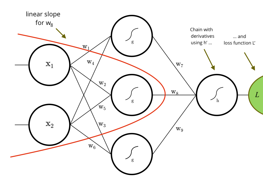
Example: Derivative for w8, built by the library.
In NeuroFlow, we work with Breeze, in particular with DenseVector[V] and DenseMatrix[V].
Let's define the XOR training data using in-line vector notation:
val xs = Seq(->(0.0, 0.0), ->(0.0, 1.0), ->(1.0, 0.0), ->(1.0, 1.0))
val ys = Seq(->(0.0), ->(1.0), ->(1.0), ->(0.0))

/*
  It's the XOR-Function :-).
  Or: the net learns to add binary digits modulo 2.
*/

net.train(xs, ys)
And then we call train on net to start.
The training progress is printed on console so we can track it.
[run-main-0] INFO neuroflow.nets.cpu.DenseNetworkDouble - [14.01.2018 22:26:56:188] Training with 4 samples, batch size = 4, batches = 1 ...
[run-main-0] INFO neuroflow.nets.cpu.DenseNetworkDouble - [14.01.2018 22:26:56:351] Iteration 1.1, Avg. Loss = 0,525310, Vector: 0.5253104527125074
[run-main-0] INFO neuroflow.nets.cpu.DenseNetworkDouble - [14.01.2018 22:26:56:387] Iteration 2.1, Avg. Loss = 0,525220, Vector: 0.5252200280272876
...
One line is printed per iteration, Iteration a.b where a is the iteration count, b is the batch and Avg. Loss is the mean of the summed batch loss Vector.
The batch count b loops, depending on the batch size, whereas the iteration count a progresses linearly until training is finished.
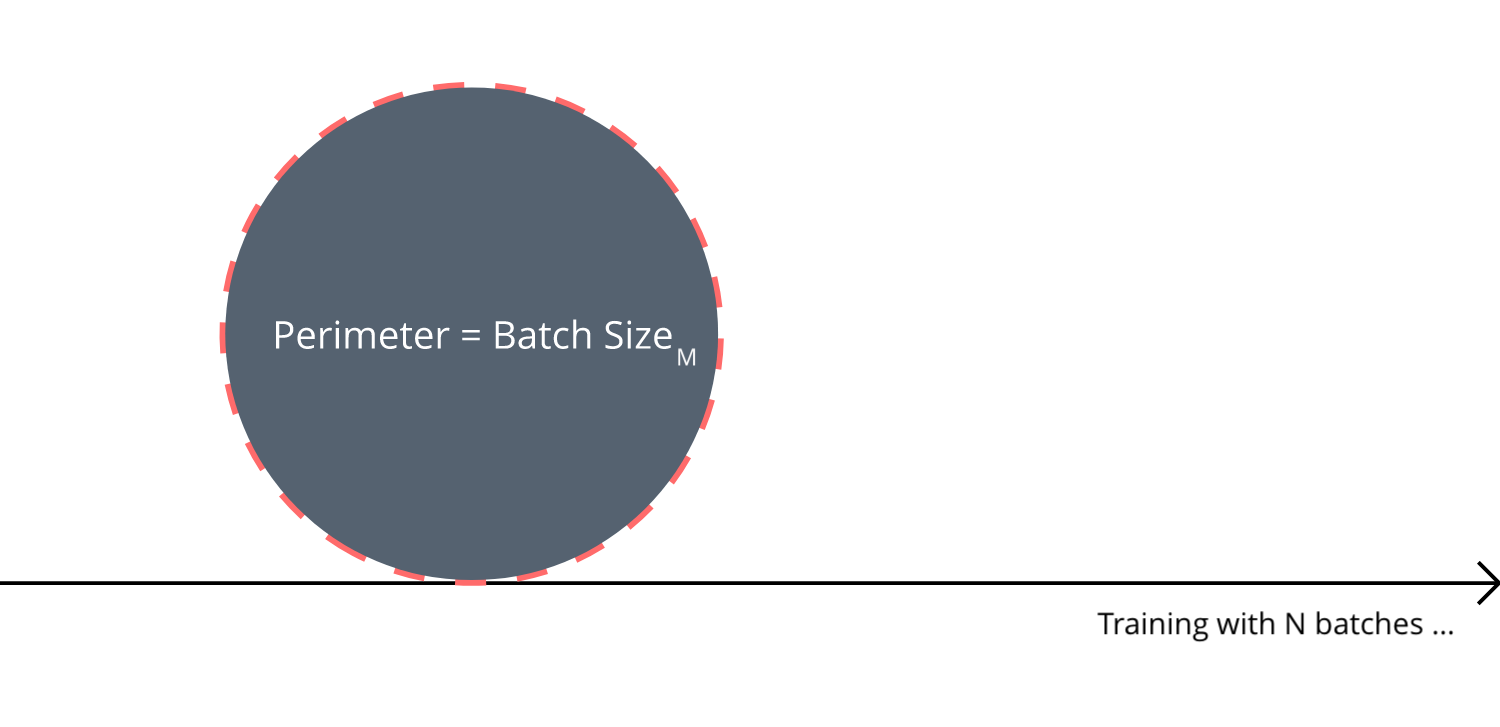
Rolling over all samples with mini-batches (M:N).
To visualize the loss function, we can iteratively append the Avg. Loss to a file with LossFuncOutput.
Settings(
  lossFuncOutput = Some(LossFuncOutput(file = Some("~/NF/lossFunc.txt")))
)
Now we can use beloved gnuplot:
gnuplot> set style line 1 lc rgb '#0060ad' lt 1 lw 1 pt 7 ps 0.5
gnuplot> plot '~/NF/lossFunc.txt' with linespoints ls 1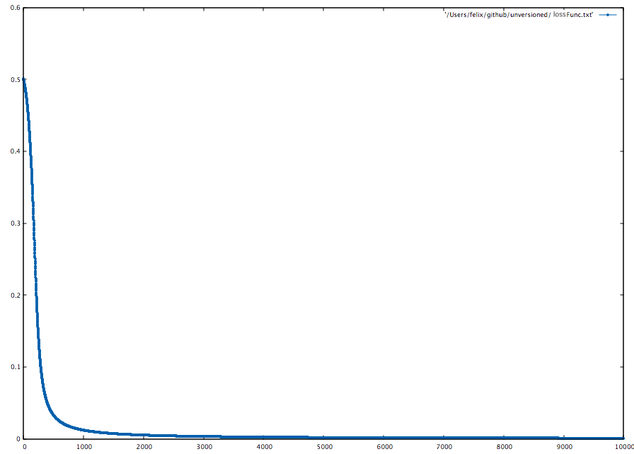
Another way to visualize the training progress is to use the LossFuncOutput with a function action: Double => Unit.
Settings(
  lossFuncOutput = Some(LossFuncOutput(action = Some(loss => sendToDashboard(loss))))
)
This function gets executed in the background after each iteration, using the Avg. Loss as input.
One example is sending the loss to a browser based grapher.
When training is done, the net can be evaluated like a regular function:
val x = ->(0.0, 1.0)
val result = net(x) // or: net.apply(x), net.evaluate(x)
println(result) // DenseVector(0.9940081702899719)
The resulting vector has dimension = 1, as specified for the XOR-example.
To compute all results of our XOR data in one step, we can use net.batchApply, which is more efficient than net.apply for each single input vector.
val res = net.batchApply(xs)
println(res.size) // = 4We can put focus on a layer and use it as the actual model output, instead of the last layer. For instance, here is a simple AutoEncoder ae:
import neuroflow.dsl.Implicits._

val b = Dense(5, Linear)
val L = Vector(23) :: b :: Dense(23, Sigmoid) :: AbsCubicError()
val ae = Network(layout = L)

ae.train(xs, xs)
It learns the input identity, but we are interested in the 5-dimensional activation from bottleneck layer b to produce a simple, compressed version of the input.
val focused = ae focus b
val result = focused(->(0.1, 0.2, ..., 0.23))
println(result) // DenseVector(0.2, 0.7, 0.1, 0.8, 0.2)
The focus on layer b gives a function, which can be applied just like the net it stems from.
The type signature of the function is derived from the focused layer's algebraic type.
Another scenario where focusing is useful is when weights are initialized, i. e. the activations of the layers can be watched and adjusted to find good values, if a JVM debugger can't be attached.
A neural net consists of matrix multiplications and function applications. Since matrix multiplication is inherently linear here, all non-linearity has to come from the cells activators. The Predefined Activators are common and should be sufficient for most data, but at times special functions are required. Here is an example how to define your own:
val c = new Activator[Double] {
  val symbol = "My non-linear activator"
  def apply(x: Double): Double = x * x
  def derivative(x: Double): Double = 2.0 * x
}
Then just drop it into a layer, e. g. Dense(3, c). Luckily, the CPU implementation is flexible to run arbitrary code.
If you need custom activators for GPU, you need to fork NF and implement them in CUDA.
You can approach a lot of challenges using the Predefined Loss Functions. However, as with the activators, at times you need
your own loss function, Y, X -> Loss, Gradient, so here is how to write one, for both CPU and GPU:
val myLoss = new LossFunction[Double] {
  def apply(y: DenseMatrix[Double], x: DenseMatrix[Double])(implicit /* operators ... */): (DenseMatrix[Double], DenseMatrix[Double]) = (loss, gradient) // CPU
  def apply(y: CuMatrix[Double], x: CuMatrix[Double])(implicit /* operators ... */): (CuMatrix[Double], CuMatrix[Double]) = (loss, gradient) // GPU
}
The targets y and predictions x are given input to produce loss and gradient, which will be backpropagated into the raw output layer.
The batch layout is row-wise, so you need to work with the matrices accordingly. Don't fear the long implicit parameters when implementing the trait,
these operators come from Breeze and should be just fine. Also look at the predefined loss functions for a starting point how to work with them.
implicit def evidence[P <: Layer, V]: (P :: myLoss.type) EndsWith P = new ((P :: myLoss.type) EndsWith P) { }To use your loss function with the front-end DSL, you need to provide evidence for compile time checks.
val L = Vector(3) :: Dense(3, Tanh) :: Dense(3, Tanh) :: myLoss
val net = Network(layout = L, settings)
Alternatively, you can work with the corresponding net implementation, passing the layout directly without any checks.
If your graphics card supports nVidia's CUDA (Compute Capability >= 3.0), you can train nets on the GPU, which is recommended for large nets with millions of weights and samples. On the contrary, smaller nets are faster to train on CPU, because while NeuroFlow is busy copying batches between host and GPU, CPU is already done.
To enable the GPU, you have to install the CUDA driver and toolkit (0.8.x). Example for Linux (Ubuntu 16.04):
curl -O http://developer.download.nvidia.com/compute/cuda/repos/ubuntu1604/x86_64/cuda-repo-ubuntu1604_8.0.61-1_amd64.deb
sudo dpkg -i ./cuda-repo-ubuntu1604_8.0.61-1_amd64.deb
sudo apt-get update
sudo apt-get install cuda
sudo apt-get install cuda-toolkit-8-0
With both driver and toolkit installed, you can import a GPU implementation for your model:
import neuroflow.nets.gpu.DenseNetwork._The library uses a hybrid approach to manage GPU RAM, both manually managed and garbage collected. Large matrices, as the batch activations or derivatives, are allocated and freed manually.
Whereas small auxiliary matrices are bound to JVM's garbage collection, which is triggered during training when free GPU RAM hits gcThreshold: Option[Long], set in bytes. The library tries to find
a good initial value, but for optimal results it has to be fine tuned to the respective graphics card.
settings.gcThreshold = Some(1024L * 1024L * 1024L /* 1G */)-Dorg.slf4j.simpleLogger.defaultLogLevel=debug # for misc runtime sys infos and gpu memory
-Xmx24G # example to increase heap size, to hold all batches in a queue on host (RAM + swap)We can save and load weights from nets with neuroflow.application.plugin.IO.
import neuroflow.application.plugin.IO._

val file = "/path/to/net.nf"
implicit val weights = File.weightBreeder[Double](file)
val net = Network(layout, settings)
File.writeWeights(net.weights, file)
val json = Json.writeWeights(net.weights)
The implicit weights to construct net come from File.weightBreeder. To save the weights back to file,
we use File.writeWeights. The weight matrices are encoded in binary format.
To write into a database, we can use Json.writeWeights to retrieve a raw JSON string and fire a SQL query with it.
Settings(
  waypoint = Some(Waypoint(nth = 3, (iter, weights) => File.writeWeights(weights, s"weights-iter-$iter.nf")))
)
It is good practice to use the Waypoint[V] option for nets with long training times. The training process can be seen as an
infinitely running wheel, and with waypoints we can harvest weights now and then to compute intermediate results. Another reason
to use it is when something crashes, saved weights allow continuation of training from a recent point. Here, every
nth = 3 step, the waypoint function is executed, receiving as input iteration count and a snapshot of the weights, which is
written to file using File.writeWeights.